
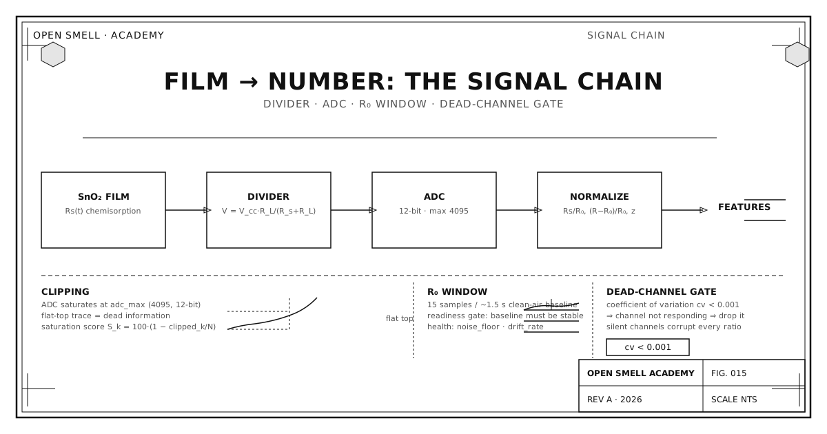
A MOX sensor does not produce numbers. It produces a resistance, which a voltage divider converts to a voltage, which an analog-to-digital converter (ADC) converts to an integer, which software converts to R_s/R_0 and then to features. Every link in that chain is a place where a naive setup quietly destroys the data. This essay walks the chain from the hot film to the feature vector, and names what can go wrong at each link.
Link 1 — The Divider
The sensor R_s(t) sits in series with a fixed load resistor R_L, and the ADC reads the midpoint:
The engineering goal is to make the change in V large enough to matter while keeping V inside the ADC's range. If R_L is much smaller than the sensor's operating resistance, the divider is stiff, V barely moves, and the whole range of sensor response maps to a handful of ADC counts. If R_L is much larger, the response swings hard but clips against the rails. Choosing R_L near the sensor's typical baseline resistance puts the operating point on the steepest part of the curve — the standard rule of thumb.
Two details deserve emphasis. First, you do not actually need to know V_cc or R_L precisely — the R_s/R_0 ratio cancels both exactly (the normalization theorem essay proves it). Second, the ADC's reference voltage and bit depth still matter, because they set the resolution of V, and therefore the smallest change in R_s you can see. A 12-bit ADC with a 3.3 V reference resolves about 0.8 mV — enough for most MOX work, and far better than the sensor's own noise.
Link 2 — The ADC and Clipping
The ADC maps the analog voltage to a fixed integer range. For a 12-bit converter, the maximum is:
Clipping happens when the signal exceeds the ADC's range: the trace flattens at 4095 (or 0) and the information in the saturated region is gone. This is not a subtle failure. It produces a flat-topped response that looks, to a downstream classifier, like a different substance — and it has happened in the OpenSmell project's own data, most memorably on a banana recording whose response slammed into the ceiling. The lesson was encoded into the quality scorer: every channel is scored for how much of its trace survived without clipping:
where clipped_k counts the samples pinned at a rail and N is the window size. A channel that clips is not adjusted after the fact; it is flagged, and the recording is treated with the suspicion it deserves. The .osmell manifest records adcBits and adcMax precisely so that any reader can reproduce the physical scale and recognize saturation.
Link 3 — Sampling Rate and Irregular Gaps
MOX transients are slow by electronic standards — rise times of seconds, recovery over tens of seconds — so a nominal sampling rate of a few hertz is usually ample. The Nyquist argument applies to the transients, not to the sensor's DC level: if your fastest meaningful feature is a 5-second rise, a 10 Hz sample stream has margin to spare.
The failure mode to fear is not low rate; it is irregular gaps. A recorder that hiccups, a logging loop that stalls, a USB bus that drops a packet — these leave holes in the timeline, and any feature computed across a hole (rise time, decay time, AUC) is silently wrong. The protocol does not trust the reported rate; it infers the median gap from the data itself, uses it as the effective sampling rate, and makes continuity one of the seven quality factors. If the median gap is inconsistent with the manifest, the record is downgraded.
Link 4 — The Baseline Window
The ratio R_s/R_0 is only as trustworthy as R_0. The framework's contract defines R_0 from a clean-air window at the start of a recording: 15 samples / roughly 1.5 seconds, aggregated by median (robust against a single glitchy sample). Two rules protect it:
- The baseline must be stable. The health dimension tracks
noise_flooranddrift_rateon the baseline window. If the baseline is itself moving (sensor still warming up, air flow changing), the recording fails the readiness gate and its features are unreliable — the capture protocol prescribes clean-air baseline → exposure → recovery, and the quality scorer refuses to pretend otherwise. - Provenance must be recorded. Was R_0 measured (explicit, from a real clean-air window) or inferred (auto, from the first samples of whatever you happened to record)? Cross-session comparability depends on the answer. The manifest carries
baseline.sourceandr0Samplesso that a later reader can tell which case they are looking at — explicit R_0 from a real clean-air window, or auto-inferred R_0 from the first samples of whatever you happened to record.
Link 5 — The Dead-Channel Gate
Some channels stop responding. A solder joint fails, an amplifier gain is mis-set, a sensor poisons — and the channel's trace becomes a flat line while the rest of the array carries on. The data still flows, which is exactly why a dead channel is dangerous: it is not absent, it is present and wrong, and it corrupts every feature that involves it — especially selectivity ratios, which divide by a per-channel response.
The gate is a coefficient-of-variation threshold. A channel whose coefficient of variation across the response is below 0.001 is not responding:
When a channel is flagged dead, the correct move is to drop it and recompute the feature set for the reduced array — not to pad it with a mean. The framework's count model (the 187-dimension essay) recomputes cleanly for any channel count, and the hardware-insufficiency gate ensures a model trained with six channels is never silently run on five by filling the gap.
The Feature Vector at the End
What arrives downstream is a normalized, quality-scored, gap-checked vector per channel: R_s/R_0 values built on a stable, provenance-recorded baseline; absolute values only where the hardware scale is meaningful; temporal and health features only where the recording actually contains the events they describe. The chain, done right, is boring. That is the point — the excitement should happen in the chemistry and the model, never in the wiring.
The Checklist
A reliable capture chain, in one list:
- Choose R_L near the sensor's baseline resistance.
- Record
adcBits/adcMax; verify you are not clipping. - Log a stable clean-air baseline first (≥15 samples).
- Fix a real sampling discipline; watch for gaps.
- Gate every channel on
cv ≥ 0.001before feature extraction. - Store raw + baseline + manifest so any consumer can re-normalize.
Sources & Further Reading
- OpenSmell master reference, §3 (
.osmellprotocol), §4.6 (the divider/normalization proof), §10.2 (the R₀ contract), §10.3 (dead-channel detection). opensmell/opensmell/mox/quality.py— the seven-factor scorer including the saturation score.opensmell/opensmell/hardware.py— theHardwareInsufficiencyWarninggate.- The
electronic-nose/build guide in the OpenSmell monorepo.