Every serious field needs a reproducible, cheap instrument that a student can build in a weekend. For digital olfaction, that instrument is the electronic nose (e-nose): an array of gas sensors whose combined response, interpreted with machine learning, produces a smell signature. This guide gets you from zero parts to a working classifier. No PCB milling, no electronics mastery—just an ESP32, some modules, and an afternoon.
What You'll Build
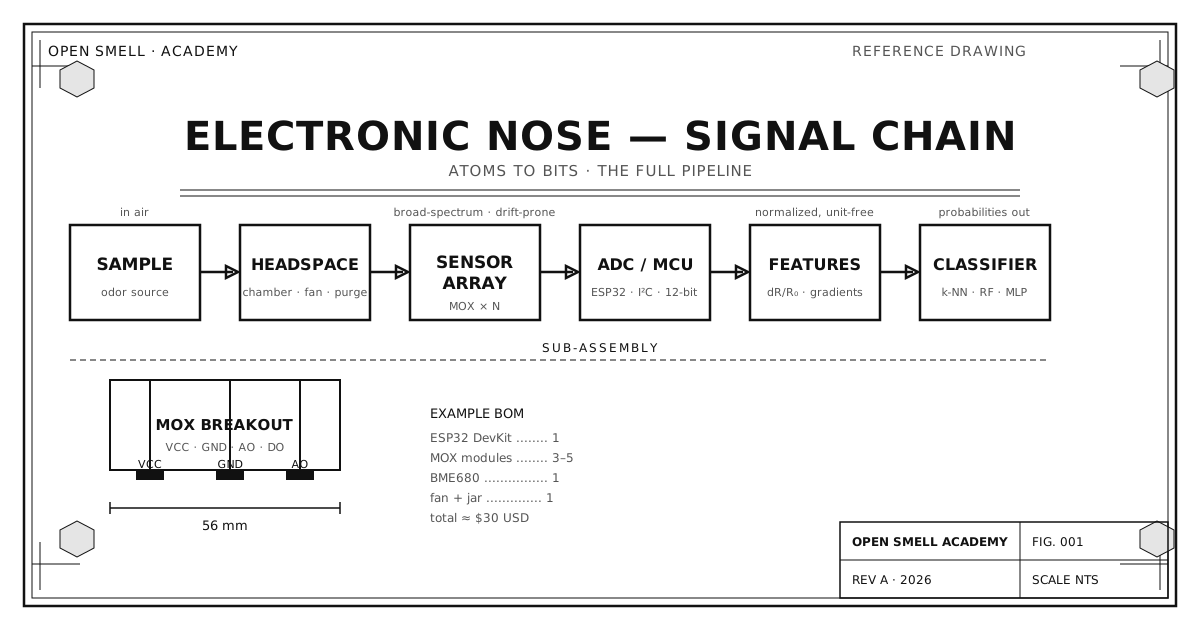
The signal chain is the whole subject of digital olfaction in miniature:
SAMPLE → HEADSPACE CHAMBER → SENSOR ARRAY ×N → ADC/MCU → FEATURES → CLASSIFIER
A fan pulls air from above an odor source into a chamber holding several MOX sensors. The microcontroller samples each sensor's analog output, normalises the readings into features, and hands them to a classifier that outputs "this is coffee" or "this is tap water." Once the plumbing works, everything above the sensors is software.
Bill of Materials
| Part | Role | Approx. cost |
|---|---|---|
| ESP32 DevKit | MCU + Wi-Fi + 12-bit ADC | $6 |
| MQ-135 | MOX, broad VOC sensitivity (ammonia, benzene, CO₂) | $3 |
| MQ-3 | MOX, alcohol-family sensitivity | $3 |
| BME680 | Temp + humidity + pressure + VOC index | $7 |
| 5 V fan + glass jar | headspace chamber + airflow | $4 |
| Breadboard + jumper wires | assembly | $5 |
| USB power bank | portable 5 V supply | $10 |
Total: ~$30–35. You can substitute any MQ module (MQ-2, MQ-7, MQ-8…); the point is diversity of sensing surfaces, not any single sensor's quality.
Why an Array?
A single MOX sensor is cross-sensitive to half the periodic table—that is its fundamental weakness and its superpower. The flaw is solved the same way biology solved it: use several broadly tuned, overlapping sensors and let the pattern across them carry the information. This is precisely the argument Persaud and Dodd made in their landmark 1982 "model nose" paper: discrimination can be achieved with broadly tuned receptors, no specific receptor required. An array of five MOX sensors, run through a classifier, vastly outperforms one "high-end" sensor on real-world discrimination tasks.
Wiring It Up
Every MQ module has four pins:
- VCC → 5 V (this powers the heater — more on that below)
- GND → GND
- AO → an analog input pin on the ESP32 (e.g. GPIO 34)
- DO → ignore this pin. The digital output is just an internal comparator and will destroy your data. Use AO.
Wire the BME680 over I²C (SDA → GPIO 21, SCL → GPIO 22 on most DevKits). Power the fan from 5 V with a transistor/MOSFET gate on GPIO 26 if you want software-controlled pumping.
Heater warning: MQ modules pull 150–800 mA and their heaters run hot (300 °C+). Always power them from the 5 V rail, never the 3.3 V logic rail, and give them a fresh warm-up of 10–30 minutes before trusting readings.
Firmware: From ADC to Numbers
The sensor output is a voltage across a load resistor, proportional to sensor resistance Rs. The quantity that actually matters is the conductance change relative to a clean-air baseline. A minimal Arduino sketch:
const int mqPins[] = {34, 35, 32, 33, 25};
const int N = 5;
float baseline[N];

void setup() {
  Serial.begin(115200);
  delay(30000); // warm-up
  for (int i = 0; i < N; i++) baseline[i] = readConductance(i);
}

float readConductance(int i) {
  float v = analogRead(mqPins[i]) / 4095.0 * 3.3;
  float rs = (3.3 - v) / v * 10.0;      // load resistor 10 kΩ
  return 1.0 / rs;                      // conductance, S
}

void loop() {
  for (int i = 0; i < N; i++) {
    float g = readConductance(i);
    Serial.print((g - baseline[i]) / baseline[i]); Serial.print(" ");
  }
  Serial.println();                     // ΔG/G₀ per sensor
  delay(100);
}
The per-sensor ΔG/G₀ vector is your first feature. It is unitless, roughly baseline-corrected, and directly comparable across devices.
The Measurement Protocol
Reproducibility is 80% of this field, and it lives in the protocol:
- Purge — run the fan on clean air for 60 s, capture fresh baseline.
- Expose — place the sample, run the fan for 20 s.
- Record — log every sensor at 10 Hz for the whole cycle.
- Purge again — 60 s clean air, let sensors recover.
- Repeat ×5 per sample, ideally across different days.
Log temperature and humidity from the BME680 alongside every reading. MOX sensors are notoriously humidity-sensitive; if you don't log it, you cannot correct it, and your model will silently learn "humidity," not "coffee."
From Raw Traces to Features
The raw time-series is high-dimensional and noisy. The OpenSmell Python SDK extracts a 187-dimensional feature framework from each exposure: per-sensor baseline-normalised response, rise and fall slopes, peak, t90 (time to 90% of max response), area under the curve, integral ratios, and cross-sensor ratios. You can start with a tiny subset yourself:
- Peak ΔG/G₀ per sensor
- Rise slope (max
dG/dtduring exposure) - t90 and recovery t50
- Humidity-normalised peak
Feed these into any off-the-shelf classifier. With five sensors and five engineered features you already have a 25-dimensional vector per measurement—plenty to separate espresso from tap water.
from sklearn.ensemble import RandomForestClassifier
from sklearn.model_selection import train_test_split

X, y = load_my_recordings()              # (n_exposures, n_features)
X_train, X_test, y_train, y_test = train_test_split(X, y, test_size=0.3)
clf = RandomForestClassifier(200)
clf.fit(X_train, y_train)
print(clf.score(X_test, y_test))
Calibration 101
A classifier tells you which smell. Calibration tells you how much. For quantitative work you need known concentrations. The empirical MOX response is a power law,
Rs / R0 = A · C^(-α)
which is linear in log-log space, so two reference points (e.g. certified gas at 10 ppm and 100 ppm) are enough to fit a rough concentration curve for a single gas. Don't over-trust it: the power law is empirical, gas-specific, and temperature-dependent.
Drift Is Real — Plan for It
The UCI Gas Sensor Array Drift dataset is the field's cautionary tale: 13,910 measurements from 10 MOX sensors over 36 months, and the sensor response drifted so much that naive classifiers trained on early months fail on later ones. Practical mitigations:
- Recompute
baseline[]on every purge. - Log batch and date and treat them as features or as a domain-adversarial problem.
- Recalibrate monthly.
- Prefer relative features (
ΔG/G₀) over raw resistance—they cancel some drift automatically.
Where to Go Next
- Flash the Osmograph firmware to get a zero-code GUI: flash, record, train, done.
- Use the OpenSmell Python SDK (
pip install opensmell) for the full 187-feature framework and pretrained classifiers. - Contribute your recordings to the OpenSmell data commons—every labeled, timestamped trace makes the open stack better for everyone.
Safety Notes
- MOX heaters reach 300 °C+; mount them clear of plastic and don't touch the mesh during operation.
- Calibrate with safe VOCs (isopropanol, ethanol, vinegar, coffee) in a ventilated space. Never sniff—or vaporize—unknown industrial chemicals.
- A "digital nose" is not a substitute for certified gas detectors in safety applications. It is a research and ML instrument. Know the difference.
Sources & Further Reading
- Persaud, K. & Dodd, G. Nature 299, 352–355 (1982).
- Figaro Engineering application notes on TGS sensors (sensitivity, drift, humidity correction).
- Vergara, A. et al. "Chemical gas sensor drift compensation using classifier ensembles." Sensors and Actuators B 166–167 (2012) — the UCI drift dataset.
- OpenSmell GitHub: https://github.com/opensmell