
The metal-oxide semiconductor (MOX) sensor is the transistor of the smell world: imperfect, ubiquitous, and quietly revolutionary. One sentence captures the whole device:
When a metal-oxide surface (usually tin dioxide, SnO₂) is heated, oxygen from the air adsorbs onto it and strips electrons from the surface. When a reducing gas arrives, it reacts with that oxygen, returns the electrons, and the material's electrical resistance drops. Measure the resistance, you measure the gas.
Everything else—the history, the engineering, the frustrations—is detail. And the details matter, because MOX sensors are simultaneously the cheapest gateway into digital olfaction and its most common source of bad data.
A Short, Dense History
The story begins in 1962, twice. In Japan, Naoyoshi Taguchi was driven by a wave of LP-gas explosion accidents sweeping the country as bottled gas reached 23 million households. After screening many oxides he landed on tin dioxide (SnO₂), filed his patent in October 1962, and commercialised the world's first gas sensor—the Taguchi Gas Sensor (TGS)—in 1968 through his company Figaro Engineering. By 1963 he had already discovered that doping the oxide with palladium dramatically improved sensitivity and selectivity. The classic TGS recipe is almost folkloric in its simplicity: a paste of tin chloride and stearic acid is painted on a substrate and fired at ~700 °C; the organic binder burns away, leaving a porous SnO₂ layer.
Meanwhile, in a Analytical Chemistry paper the same year, Seiyama and Kato demonstrated the first thin-film ZnO gas sensor based on the same resistance-change mechanism. Two independent discoveries, one physics.
Decades later, in 1982, Persaud and Dodd wired a few of these devices together, called it a "model nose," and showed that broadly tuned sensors plus pattern recognition could discriminate smells. The e-nose was born—and MOX sensors became its default sensor because they are cheap to make and sensitive to almost everything volatile and reducible.
The Physics: Oxygen Is the Gatekeeper
SnO₂ is an n-type semiconductor with a wide band gap (~3.6 eV). Heated to 300–450 °C, its surface chemisorbs oxygen as negatively charged species (O₂⁻, O⁻, O²⁻ depending on temperature). Each adsorbed oxygen ion captures an electron from the conduction band, depleting the near-surface region of charge carriers. At the junctions between sintered grains, this depletion creates energy barriers that electrons must cross—so the sensor sits in a high-resistance state.
Then a reducing gas—ethanol, CO, hydrogen, methane—arrives and reacts with the adsorbed oxygen:
CO + O⁻ → CO₂ + e⁻
The released electron returns to the conduction band, the barriers collapse, and resistance drops. The size of the drop scales with gas concentration. Note the asymmetry that catches beginners: oxidising gases like NO₂ or ozone steal electrons, so resistance rises. There is no universal sign convention—always check the datasheet.
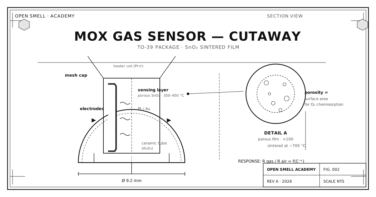
Anatomy of a TGS Sensor
A classic tubular TGS (like the MQ modules) is remarkably low-tech:
- Sensing layer — porous SnO₂ (or doped SnO₂: Pd, Pt) sintered at ~700 °C.
- Electrodes — gold or platinum wires measuring the film's resistance.
- Heater — a platinum–iridium coil running through the ceramic tube, held at 300–450 °C (older units draw ~150–800 mW; modern MEMS versions like the TGS8100 drop to ~15 mW).
- Ceramic tube / substrate — alumina (Al₂O₃), chosen for thermal stability.
- Mesh cap + metal can — mechanical protection; the can keeps flame from propagating if a combustible mix ignites near the heater.
The geometry is pure engineering craft: you want porosity (maximises the surface available for chemisorption) but you also want mechanical strength. Every manufacturer has their own sintering recipe, which is why "two MQ-135s are not two MQ-135s."
The Response Model
For a fixed temperature, the empirical response is a power law:
Rs / R0 = A · C^(-α)
where Rs is resistance in the gas, R0 the clean-air baseline, C the concentration, and A, α empirical constants. Take the log of both sides and you get a straight line—this is why MOX datasheets plot log–log "sensitivity curves" and why you fit calibrations in log space. The exponent α is typically ~0.5, which tells you the sensor is nonlinear and saturating: it can detect a few ppm of ethanol and a few hundred ppm of methane, but its dynamic range is only a few decades.
Dynamics: Not Just How Much, But How Fast
Response dynamics carry information too. t90 (time to reach 90% of the steady-state response) and recovery time differ between gases, and temperature modulation—pulsing the heater between 200 °C and 400 °C—changes the selectivity profile over time, creating a pseudo-spectrum that can be fed to a classifier. This is a cheap trick that meaningfully improves discrimination and is a great first experiment.
The Selectivity Problem (and Why Arrays Exist)
The dirty secret: an MOX sensor cannot tell CO from ethanol by itself. Both are reducing gases; both drop the resistance. Dopants buy partial specificity (Pd:CO, Pt:CH₄), but broad cross-sensitivity is intrinsic. The field's answer, since Persaud and Dodd, is arrays: run N sensors with overlapping response profiles and let pattern recognition do the separation. A single MOX sensor is a gas alarm; an array of MOX sensors is an instrument.
Drift, Humidity, and Poisoning
Three enemies, all well documented:
- Humidity — water vapour changes the oxygen-adsorption equilibrium and shifts the baseline by tens of percent. Compensate with a co-located humidity sensor (this is exactly why the OpenSmell stack mandates logging T/RH).
- Drift — long-term slow change in the sensing film (recrystallisation, contamination). The UCI drift dataset documented failures of naive models over 36 months. Mitigate with periodic recalibration and relative features.
- Poisoning — silicone vapours (from sealants, lubricants) can permanently deactivate the surface. Keep the sensor away from fresh silicone.
Reading One Properly
A five-point checklist before you trust any MOX number:
- Warm up ≥ 10–30 minutes until the baseline is stable.
- Express results as
ΔG/G₀orRs/R0— never raw voltage. - Log temperature and humidity.
- Calibrate in log space against known concentrations.
- Treat "ppm" estimates as ±factor-of-two at best unless you have certified references.
MOX sensors are not precise. They are cheap, fast, and information-rich—and with an array and a classifier, that is a winning combination. Most of the hard problems in digital olfaction are not solved by a better sensor; they are solved by better use of the sensors that cost three dollars.
Sources & Further Reading
- Taguchi, N. U.S. Patent 3,631,436, "Gas detecting devices" (filed 1967, granted 1971); U.S. Patent 3,625,756 (manufacture of the porous element).
- Seiyama, T. & Kato, A. "A new detector for gaseous components using semiconductor thin film." Analytical Chemistry 34, 1502–1503 (1962).
- Persaud, K. & Dodd, G. Nature 299, 352–355 (1982).
- Korotcenkov, G. "First fifty years of chemoresistive gas sensors." Chemosensors 3, 1 (2015).
- Figaro Engineering, History and TGS technical application notes: https://www.figaro.co.jp
- Vergara, A. et al. UCI gas sensor drift dataset, Sensors and Actuators B (2012).