
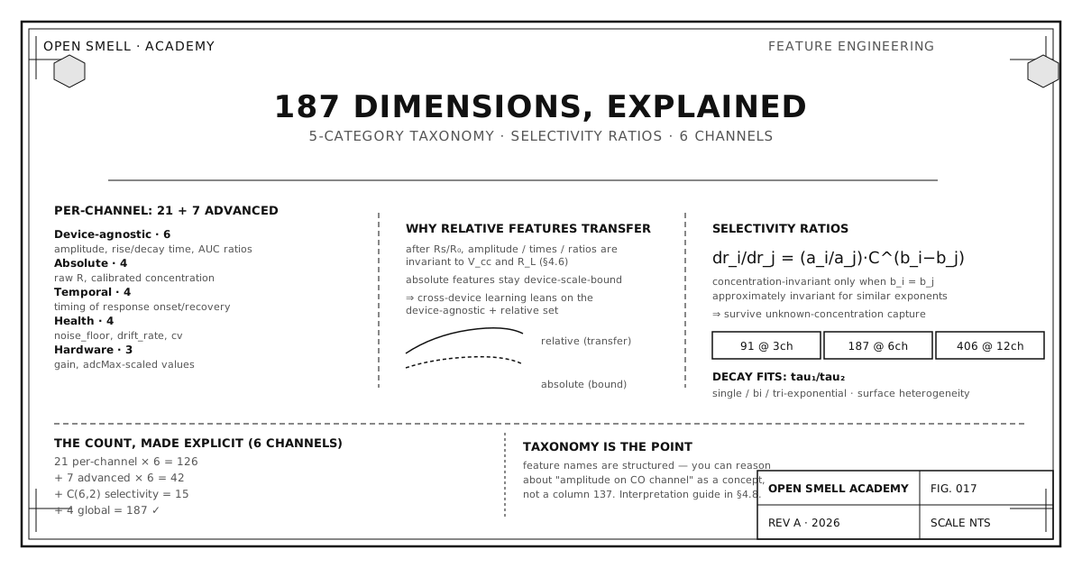
A raw MOX recording is a table of voltages: thousands of rows, a handful of columns. No classifier eats that directly — and even if it could, the result would be a model that memorizes a particular rig, a particular day, and a particular timing. The OpenSmell framework's answer is a structured feature taxonomy: a fixed, named set of features that turns any recording into a vector whose entries have meanings you can reason about.
At six channels, that vector has 187 dimensions. This essay explains the taxonomy, where every one of those numbers comes from, and which of them survive the trip to a different device.
The Five-Category Spine
The per-channel features are organized into five categories. The categories are not cosmetic; they encode why a feature behaves the way it does:
| Category | Per channel | What it captures | Transfer behaviour |
|---|---|---|---|
| Device-agnostic | 6 | amplitudes, rise/decay times, AUC ratios | transfers (relative) |
| Absolute | 4 | raw resistance, calibrated concentration | bound to this device |
| Temporal | 4 | onset/recovery timing, latency | transfers (relative) |
| Health | 4 | noise floor, drift rate, cv | transfers (diagnostics) |
| Hardware | 3 | gain-scaled, adcMax-scaled values | bound to this hardware |
The two columns on the right are the reason the taxonomy exists at all. Relative features transfer; absolute features do not. An amplitude expressed as a ratio of its own baseline survives a different supply voltage, a different gain, and (after R_s/R_0) a different load resistor, because the electronics cancel out (the normalization theorem essay). A raw resistance in kilohms is a statement about one particular board on one particular day. Keeping the two categories distinct is what lets a model trained on rig A have any hope of being probed on rig B — and, just as importantly, lets you know exactly which part of the model is hostage to rig A.
The Count, Worked Out
The arithmetic behind "187" is transparent. Per channel there are 6 + 4 + 4 + 4 + 3 = 21 standard features. On top of those, each channel contributes 7 advanced features (saturation index and multi-exponential decay constants — the decay model is its own essay). Then the array contributes cross-channel features, and the whole recording contributes global features:
| Group | Per channel | N = 3 | N = 6 | N = 12 |
|---|---|---|---|---|
| Device-agnostic | 6 | 18 | 36 | 72 |
| Absolute | 4 | 12 | 24 | 48 |
| Temporal | 4 | 12 | 24 | 48 |
| Health | 4 | 12 | 24 | 48 |
| Hardware | 3 | 9 | 18 | 36 |
| Advanced | 7 | 21 | 42 | 84 |
| Selectivity ratios | N(N−1)/2 | 3 | 15 | 66 |
| Global | — | 4 | 4 | 4 |
| Total | 91 | 187 | 406 |
The N(N−1)/2 term is where the array's cross-sensitivity becomes a feature (next section). Note the growth pattern: the feature count is quadratic in channels, because the selectivity-ratio term grows with pairs — but as the sensor count essay showed, the effective dimensionality grows only logarithmically. You get more columns per channel, not more independent information per channel.
Selectivity Ratios: The Array's Signature Feature
Two channels i and j respond to a gas through their own power laws. Their ratio is
This single expression does the heavy lifting of array-based identification. When the exponents match (b_i = b_j), the ratio is independent of concentration — a pure fingerprint of the substance that works whether the recording captured 5 ppm or 500 ppm. When they differ, the ratio still varies with C, and the framework says so explicitly rather than pretending otherwise.
This is the feature that makes a nose out of sensors that are individually unselective (the band bending essay). And because it is a ratio of per-channel responses, it is also the feature most sensitive to a dead channel — which is why the dead-channel gate (cv < 0.001) runs before the ratio computation, not after.
Advanced Features: Saturation and Decay
Two per-channel advanced groups deserve their own mention because they encode physical events rather than statistics.
- Saturation index measures how close a response came to the ADC rail (and, separately, to the sensor's own response saturation). A saturated channel's other features are unreliable, so saturation index is designed to be checked first — the framework's interpretation guide routes feature-selection decisions through it.
- Multi-exponential decay constants (single, bi-, tri-exponential fits to the recovery phase) capture surface heterogeneity: a surface with one dominant binding site decays as a single exponential; multiple sites produce a sum. The recovered time constants τ₁, τ₂ are physically meaningful and transfer across sessions better than raw recovery slopes. The equal-cost caveat is on record: MINPACK-style fits can land in different local minima for equally good errors, so the constants are stable for comparison within one fitting pipeline, not infinitely reproducible across pipelines.
Global Metrics
Four features summarize the whole recording: total active channels, overall signal-to-noise, average drift over the session, and a compact "which channels fired" mask. These are the first features a clustering step looks at, and the cheapest to compute from any container.
What the Numbers Are Actually For
A structured taxonomy changes how you work with a model in three practical ways:
- You can reason about features by name. "Amplitude on the CO channel" is a concept; "column 137" is not. When a classifier leans on one feature, you can ask why it makes sense — or notice that it is a hardware-bound absolute feature that will not survive a rig change.
- You can drop a whole category cleanly. Recording without a recovery phase? Drop the temporal and decay features rather than feeding in garbage. Unknown concentration? The framework warns that selectivity ratios degrade unless exponents match. The taxonomy makes these decisions structural instead of ad hoc.
- Transfer is scoped by feature category. The cross-device story of this framework is precisely the category story: device-agnostic features transfer, absolute and hardware features do not, and per-rig calibration is what upgrades a device-agnostic model into a cross-rig one (the calibration essay).
The Bottom Line
Every one of the 187 features has a name, a category, a transfer class, and a failure mode — the feature space is auditable. That is what separates a feature extractor from a feature framework, and it is why the same taxonomy appears, 1:1, in the Python SDK and the TypeScript web stack, kept equal by tests.
Sources & Further Reading
- OpenSmell master reference, §4 (the full 187-dimension framework), §4.7 (feature counts), §4.8 (interpretation guide), §4.9 (use-case recipes).
opensmell/opensmell/mox/features.py—extract_all_framework_features.- OpenSmell master reference, §5 (multi-exponential decay model) for the τ₁/τ₂ details.
- The normalization theorem essay — for why device-agnostic features transfer.