Here is the position at the center of this essay: a MOX sensor does not measure concentration, it measures resistance, and the mapping between the two contains two unknowns that differ for every unit you buy. Calibration is the procedure for turning resistance readings into quantities you can report. This essay gives you the procedure, the arithmetic, and — most importantly — the measured error bars.
What You Are Calibrating
The sensor's response to a target gas at concentration C is
with two per-channel constants: a (the overall gain) and b (the concentration response). Both are unit-specific — manufacturing tolerance alone is 20–30% — and both drift with temperature and age. Calibration means measuring (a, b) for your channel, your gas, on your rig.
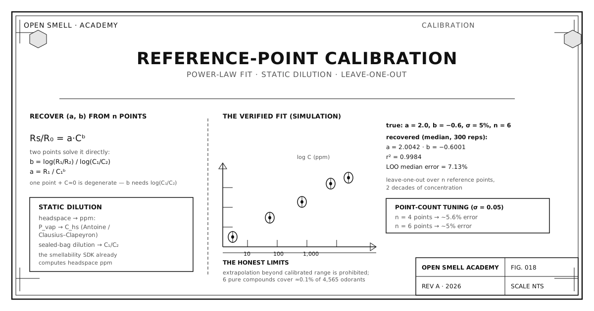
Two reference points are the mathematical minimum, because the system has exactly two unknowns:
But the minimum is not the recommendation. Note what the first equation needs: two genuinely different concentrations. The denominator log(C₁/C₂) is what carries the information, so a calibration that spans a tiny concentration range — or tries to use C = 0 as a reference — produces a b that is noise. The practical rule is to span at least two decades of concentration and to fit (a, b) by log–log ordinary least squares across all reference points, not just two. More points average out the sensor noise; two points do not.
Where Reference Concentrations Come From
You need known C values to feed the fit, and you get them without a gas chromatograph:
- Headspace from vapor pressure. A pure liquid's saturated headspace concentration follows from its vapor pressure (Antoine/Clausius–Clapeyron) at your temperature — the same thermodynamics the SMILES to smell essay uses. Fill a sealed container, let it equilibrate, and the gas above it has a computable ppm.
- Sealed-bag dilution. Dilute the saturated headspace with clean air in known volume ratios to produce a ladder of concentrations C₁, C₂, C₃, … spanning your two decades. The ratio C₁/C₂ is set by volumes, which you control precisely — which is exactly what the b-estimator needs.
Neither method claims laboratory-grade metrology. Both claim the thing that matters for calibration: known, controllable, reproducible concentration ratios.
The Verified Error Bars
The method's credibility comes from a numerical falsification that was actually run: simulate a sensor with known truth, add realistic noise, and see how well calibration recovers the truth. The setup — a = 2.0, b = −0.6, measurement noise σ = 5%, n = 6 reference points across two decades, 300 repetitions — produced:
- recovered a = 2.0042 (true 2.0)
- recovered b = −0.6001 (true −0.6)
- fit R² = 0.9984
- leave-one-out median concentration error ≈ 7.1%
The method is unbiased: it does not systematically drift the constants, and the LOO error — predicting each reference point from the other five — is the number to quote when someone asks "how wrong is this calibration?"
The data budget matters as much as the fit. The point-count grid shows how error falls as you add references:
| Reference points | σ = 5% | σ = 10% |
|---|---|---|
| 4 | 9.5% | 19.0% |
| 5 | 8.2% | 16.2% |
| 8 | 6.6% | 13.1% |
The flagship recovery run above (6 points, σ = 5%, two decades, 300 reps) measured 7.1% LOO error, consistent with this grid.
Two rules fall out. Span sets the reportable range, not the in-range accuracy: extrapolating past the top calibrated ppm is penalized, so the calibration's legal range is exactly the range you measured. And noise compounds fast: a rig with within-session scatter of σ ≈ 12% — the level measured on the OpenSmell rig — will show ~20–40% concentration error on a single exposure, which is why the protocol prescribes multiple replicates (four per point pulls the effective σ back toward 5%).
The One-Point Trap and the Affine Dead End
Two alternative "shortcuts" keep failing, and the project has the measurements to say so rather than assume so.
The one-point "M" calibration — scale everything by a single exposure to make one known substance match — fails structurally. In the measured experiments it restored +0.0 percentage points on the full model and even degraded some settings, because one point cannot pin down b, and b is where the concentration behavior lives. The pure-gain case (where one point is mathematically sufficient) is real but almost never the actual situation; real drift is exponent-shaped, not gain-shaped.
Affine calibration — learn a linear map from device A's feature space to device B's (3→6 channel) — failed outright on real cross-device data, going from 47% to 33% accuracy. A linear map cannot create dimensions that do not exist (see the sensor count essay), and the features that matter do not transform affinely across units. Both dead ends point the same way: measure (a, b) on each rig, per substance.
The Sanctioned Protocol
Putting it together, the reference-point protocol is:
- Choose a target substance and a reference method (headspace or sealed-bag dilution).
- Build a concentration ladder spanning ≥ 2 decades (e.g., 10, 30, 100, 300, 1000 ppm).
- Record clean-air baseline → exposure → recovery for each point, following the capture protocol.
- Fit (a, b) per channel by log–log OLS across all points.
- Report LOO error alongside the fit, and state the calibrated span.
- Record the result in the manifest:
{ a, b, reference_substance, reference_ppm, date, method }— so every future reader knows the constants are measured, not nominal.
The SDK implements the whole pipeline — fit_power_law, loocv_power_law, invert_concentration, build_calibration_payload — and the calibration contract round-trips through the .osmell manifest. The only missing piece in the project is real labeled-ppm recordings from hardware, which is a data problem, not a method problem.
The Limit: Anchors Are Not Universes
Calibration is a reference-point strategy, not a universal map. Six pure reference compounds — even well chosen — cover roughly 0.1% of the ~4,565 odorants in a standard reference corpus (a convex-hull analysis of the measured result). The consequence is operational, not philosophical: you calibrate for the substances you actually care about, per rig, and you ship a contribution loop so the community's reference library grows — rather than pretending six bottles can span the smell of the world.
The payoff is that calibrated readings become comparable artifacts: two rigs, calibrated against the same ladder, produce concentration estimates that can be pooled. That is the entire foundation the interoperability essay demands, and it is reachable with a bottle, a bag, and a spreadsheet.
Sources & Further Reading
- OpenSmell master reference, §4.6 (two-point derivation), §10.10 (calibration hooks and the falsification results), §8.7 (the reference-point calibration method).
research/calibration-experiments/reference-point-calibration/results.json— the verified a = 2.0042 / b = −0.6001 / LOO ≈ 7.1% numbers.opensmell/opensmell/calibration.py—fit_power_law,loocv_power_law,invert_concentration,build_calibration_payload.- The interoperability essay — why calibration is the only sanctioned route to cross-device quantification.