
If you have held a cheap gas sensor, you have held a small ceramic tube wrapped in a sintered film of tin dioxide (SnO₂), a coil of platinum–iridium wire inside to heat it to somewhere around 350–450 °C, and a pair of electrodes measuring resistance across the film. That is a MOX sensor — a metal-oxide semiconductor chemiresistor. It is the workhorse of hobbyist and industrial gas sensing alike, and it is the sensor behind most electronic noses.
This essay is about what actually happens inside that film. Not because the chemistry is interesting for its own sake, but because every practical decision about an electronic nose — how many sensors to buy, how to arrange them, what calibration can and cannot promise, why drift happens — is a direct consequence of this surface chemistry. Read this once and the rest of the field makes sense.
What a MOX Sensor Actually Is
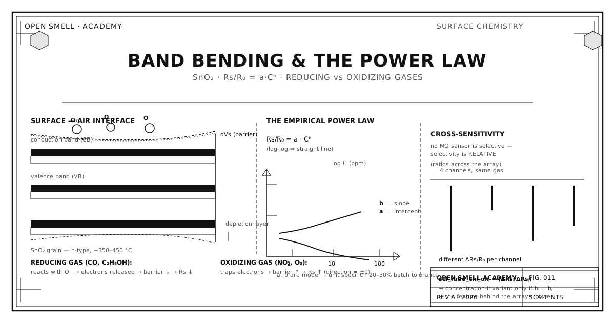
A MOX sensor is built around a thick film of metal oxide, most commonly SnO₂, deposited on a ceramic tube or micro-hotplate and heated from below. In clean air the surface of the film chemisorbs oxygen. Oxygen molecules pull electrons out of the conduction band of the oxide, forming adsorbed species (O₂⁻, O⁻, and O²⁻ depending on temperature) and leaving a region near the surface depleted of charge carriers. The resistance of the film is dominated by the potential barriers that this depletion creates at grain boundaries — the contact points between individual SnO₂ crystallites where the depleted zones overlap.
That is the central fact of MOX sensing: the resistance you measure is controlled by the height of an energy barrier at the surface, and that barrier is controlled by what is adsorbed there. A gas sensor is therefore not measuring "how much gas is present" directly. It is measuring how the adsorbed-oxygen population — and the resulting barrier height — is perturbed by the gases in the air.
Band Bending: The Surface as an Interface
In solid-state terms, the physics is band bending. Imagine the conduction band of the SnO₂ crystal as a horizontal line at a given energy. Near the surface, adsorbed oxygen traps electrons, so the density of free carriers drops and the bands bend upward toward the surface. The result is a barrier qV_s at every grain boundary that electrons must cross to carry current. When a reducing gas arrives, it reacts with the adsorbed oxygen (for example, CO + O⁻ → CO₂ + e⁻), releasing an electron back into the conduction band. The depletion shrinks, the barrier drops, and the measured resistance falls.
An oxidizing gas does the opposite. NO₂ and O₃ trap additional electrons directly at the surface, deepening the depletion, raising the barrier, and increasing resistance.
We therefore need a sign convention. Let us define the sensor's response direction as
Reducing gases (CO, ethanol, most VOCs) give a negative direction — resistance decreases. Oxidizing gases (NO₂, O₃) give a positive direction — resistance increases. The framework treats this as a first-class feature, because a substance that raises resistance is telling you something chemically different from one that lowers it, and mixing the two up silently destroys classifiers.
The Empirical Power Law
For a single target gas at concentration C, the sensor's response follows an empirically robust relationship — a power law:
where R_s is the resistance in the presence of the gas, R_0 is the resistance in clean air, and a and b are sensitivity constants. On a log–log plot this is a straight line:
The exponent b is the slope — the concentration response of the sensor. The constant a is the intercept — the overall gain. Both are specific to a given sensor model and to a given target gas, and both vary from unit to unit with a manufacturing tolerance of roughly 20–30%. That variability, more than anything else, is why electronic noses need per-device calibration, a theme developed in the companion essay What a Normalized Reading Can and Cannot Mean.
Why a power law? In the simplest physical picture, the resistance varies exponentially with barrier height, and the barrier height varies logarithmically with the partial pressure of the reducing gas via the adsorption isotherm. Two logarithms compose into a power law. Real sensors deviate from a clean power law at very low and very high concentrations, but over one to three decades of concentration — the range a practical sensor is used in — the power law is a dependable engineering approximation.
Where a and b Come From
Two known concentrations are enough to recover both constants. Measure the response at C₁ and C₂:
Note the shape of the denominator in the first equation: b is only defined when the two reference concentrations are different. Calibrating with one point and an assumed "zero" point is degenerate, because log(C₁/C₂) blows up as C₂ → 0. That single fact explains why "one-point calibration" attempts in this field produce unusable results, and why the sanctioned reference-point protocol always spans at least two decades of concentration. The Reference-Point Calibration essay develops this properly.
Cross-Sensitivity: Selectivity Is a Ratio, Not a Switch
Here is the uncomfortable truth that shapes all of e-nose engineering: no MOX sensor is selective. A sensor marketed as "alcohol sensor" will also respond to CO, methane, hydrogen, and most other reducing gases. Its name reflects the gas it was characterized against, not a physical lock on that molecule.
What an array gives you is not selectivity per sensor but a relative pattern across sensors. If channel i responds to a gas with constants (aᵢ, bᵢ) and channel j with (aⱼ, bⱼ), then the ratio of their responses to the same gas is
Two consequences fall directly out of this equation.
First, the ratio is concentration-invariant only when bᵢ = bⱼ. If two channels have the same exponent, their ratio is a pure number that identifies the gas regardless of how much of it is present — a property the feature framework exploits. If the exponents differ, the ratio silently varies with concentration, and a classifier trained at one concentration level degrades at another.
Second, this is the mathematical reason cross-sensitivity is a feature of an e-nose and not a bug. A "selective" single sensor gives you one scalar — a detector, not a nose. An array whose sensors overlap in sensitivity but differ in the details (aᵢ, bᵢ) gives you a vector in a space where gases land in different places. That vector is what pattern recognition works on. The selection rules for arrays — see How Many Sensors Make a Nose? — follow directly: what matters is the diversity of the sensitivity profiles, not the number of sensors.
The Interference Budget
The same surface chemistry that responds to your target gas responds to other things in the environment, and a practical e-nose must budget for them explicitly.
- Humidity. Water vapor is a reducing-adjacent interferent that affects every SnO₂ sensor. Because it is common-mode across the array (it changes all channels in the same direction), it effectively consumes one whole dimension of your discriminative space — an array with N sensors behaves more like an array with N − 1 degrees of freedom in a humid environment. Differential measurement or per-recording z-score normalization is essential.
- Temperature. MOX sensitivity shifts by roughly 2–5% per degree Celsius. Small temperature swings read like small gas events. The mitigation is not exotic compensation but disciplined capture: log temperature, keep the environment stable, and never trust a reading taken while the rig is still warming up.
- Air flow and pressure. These change how quickly molecules reach the surface and how the film equilibrates, distorting the temporal features (rise time, decay time) that classifiers lean on. The capture protocol — clean-air baseline → exposure → recovery, with the sensor held still — exists to make these variables reproducible.
- Oxygen itself. The sensor's entire operating point depends on the ambient oxygen level. At drastically reduced oxygen (inert gas or altitude), the baseline R₀ moves and the power law shifts. A MOX sensor is fundamentally an oxygen-and-adsorbate instrument.
None of these are surprises if you start from the band-bending picture. All of them are surprises if you treat the sensor as a black box that "outputs ppm."
Drift and Poisoning
Two degradation modes dominate field failures, and both are surface phenomena.
Baseline drift is a slow change in R₀ over weeks and months — sintering of the film, slow migration of surface species, accumulated contamination. The fix is operational: periodic re-zeroing against reference clean air, and always expressing readings relative to a freshly measured R₀ rather than an absolute resistance.
Poisoning is the catastrophic cousin. H₂S, siloxanes (found in many household products), and halogens bind irreversibly to the SnO₂ surface and permanently degrade sensitivity. A clean-air MOX sensor lives one to three years; in a harsh environment, weeks. There is no recovery from poisoning — the sensor must be replaced.
What This Means for Arrays
Everything in this essay compresses into a few engineering rules:
- The signal is Rs/R₀, a ratio, never raw resistance.
- Direction (±) is a first-class feature: reducing vs oxidizing gases are different physics.
- Response follows a·C^b; a and b are per-model, per-gas, and per-unit.
- "Selectivity" only exists as ratios across channels, and only meaningfully when exponents are similar.
- Humidity, temperature, and flow are not noise to average away; they are variables to control or log.
- Drift and poisoning are surface processes; they respond to protocol (baseline windows, clean-air references, environmental discipline), not to software patches.
An electronic nose is a chemical instrument whose physics is well understood. The reason this field is hard is not mystery — it is variability: a, b, drift, humidity, batch. The reason it is possible is that the physics is stable enough to be modeled, normalized, and calibrated. The remaining essays in this series show how that is done, with the numbers to prove it.
Sources & Further Reading
- OpenSmell master reference, §4.6 (the Rs/R₀ normalization proof) and §6 (sensor theory).
opensmell/opensmell/mox/quality.pyand theelectronic-nose/build guide in the OpenSmell monorepo.- Gardner & Bartlett, Sens. Actuators B 18 (1994) — electronic nose fundamentals.
- Marco & Gutierrez-Galvez, Sens. Actuators B 166–167 (2012) — signal and data processing for MOX arrays.